Basic
Import Numpy
import numpy as np
Initialize An Array
a = np.array([4,5,6])
print(a.dtype)
print(a.shape)
print:
int32
(3,)
2-D Array
b = np.array([[4,5,6],[1,2,3]])
print(b.shape)
print(b[0][0],b[0][1],b[1][1])
print:
(2, 3)
4 5 2
Zeros, Ones , Eyes & Random
Caution: Only One Arg of Shape in .Eyes()
a  = np.zeros((3,3),dtype=int)
print("a:\n",a)
b = np.ones([4,5])
print("b:\n",b)
c = np.eye(4,dtype=int)
print("c:\n",c)
d = np.random.randint(6,15,6) # random 6 integers from 6 to 14
d = d.reshape((3,2))
print("d:\n",d)
print:
a:
 [[0 0 0]
 [0 0 0]
 [0 0 0]]
b:
 [[1. 1. 1. 1. 1.]
 [1. 1. 1. 1. 1.]
 [1. 1. 1. 1. 1.]
 [1. 1. 1. 1. 1.]]
c:
 [[1 0 0 0]
 [0 1 0 0]
 [0 0 1 0]
 [0 0 0 1]]
d:
 [[ 9 13]
 [12 11]
 [ 6 13]]
More about Random
d = np.random.rand(6)
d = d.reshape((3,2))
print("d:\n",d)
e = np.random.rand(3,4)
print(e)
print:
d:
 [0.59773306 0.00885552 0.64095474 0.07965694 0.80679749]
[[0.78392635 0.44353436 0.1636798  0.80779348]
 [0.19202358 0.47410758 0.49104906 0.6336175 ]
 [0.71719759 0.09642529 0.69724053 0.06804706]]
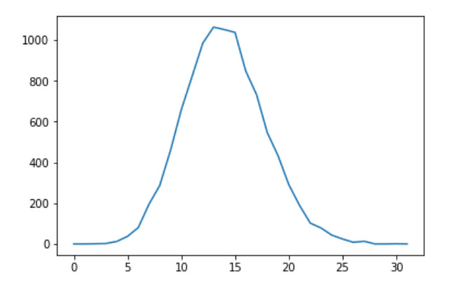
Distribution
- prng.chisquare(1, size=(2, 2)) # 卡方分布
- prng.standard_t(1, size=(2, 3)) # t 分布
- prng.poisson(5, size=10) # 泊松分布
e=np.random.poisson(14,size=10000)
#print(e)
l = np.zeros(2*16,dtype=int)
xxx = np.arange(0,2*16,1)
for t in e :
    l[t]+=1
print(l)
import matplotlib.pyplot as plt
plt.plot(xxx,l)
plt.show()
Print:
[   0    0    1    2   12   37   80  195  287  459  658  821  985 1064
 1052 1038  848  733  546  433  291  189  102   78   43   24    8   13
    0    0    1    0]
Index
a = np.array([[1, 2, 3, 4], [5, 6, 7, 8], [9, 10, 11, 12]] )
print("a:\n",a)
print("(2,3) ",a[2][3],"\n(0,0) ",a[0][0])
print:
a:
 [[ 1  2  3  4]
 [ 5  6  7  8]
 [ 9 10 11 12]]
(2,3)  12
(0,0)  1
Copy Partly From 2-d Array
b = a[0:2,2:4]

print("b:\n",b)
print:
b:
 [[3 4]
 [7 8]]
Copy the last 2 row of a to c
c = a[1:3][:]
print("c:\n",c)
print("last element of 1st row of c: ",c[0][-1])
print:
c:
 [[ 5  6  7  8]
 [ 9 10 11 12]]
last element of 1st row of c:  8
Print 3 element (0,0) (1,1)(2,0)
a = np.array([[1, 2], [3, 4], [5, 6]])
print(a[:,0])
print(a[np.arange(3),[0,0,0]])
print(a[[0,1,2],[0,1,0]])
print:
[1 3 5]
[1 3 5]
[1 4 5]
print (0,0),(1,2),(2,0),(3,1)
a =np.array([[1, 2, 3], [4, 5, 6], [7, 8, 9], [10, 11, 12]])
print(a[[0,1,2,3],[0,2,0,1]])
b = np.array([0, 2, 0, 1])
print(a[np.arange(4), b])
print:
[ 1  6  7 11]
[ 1  6  7 11]
Add the 4 elements above with 4
a[np.arange(4),b] += 10
print(a[np.arange(4),b] )
print:
[11 16 17 21]
Operation
add & +
x = np.array([[1, 2], [3, 4]], dtype=np.float64)
y = np.array([[5, 6], [7, 8]])
print(x+y)
print(np.add(x,y))
print:
[[ 6.  8.]
 [10. 12.]]
[[ 6.  8.]
 [10. 12.]]
substract & -
print(x-y)
print(np.subtract(x,y))
print:
[[-4. -4.]
 [-4. -4.]]
[[-4. -4.]
 [-4. -4.]]
multiply V.S. dot
print(x*y)
print(np.multiply(x, y) )
print(np.dot(x, y) ) #矩阵乘积
xx =np.array([[1,2,3],[1,2,3]])
yy =np.array([[1,2,3],[1,2,3]])
print(xx.shape)
yy=yy.transpose()
print(yy.shape)
print(np.dot(xx,yy) ) #矩阵乘积
print:
[[ 5. 12.]
 [21. 32.]]
[[ 5. 12.]
 [21. 32.]]
[[19. 22.]
 [43. 50.]]
(2, 3)
(3, 2)
[[14 14]
 [14 14]]
divide
print(np.divide(x,y))
print(np.divide(y,x))
print:
[[0.2        0.33333333]
 [0.42857143 0.5       ]]
[[5.         3.        ]
 [2.33333333 2.        ]]
sqrt
print(np.sqrt(x))
print:
[[1.         1.41421356]
 [1.73205081 2.        ]]
sum
print("x:\n",x)
print("Mean : ",np.mean(x))
print("0 axis: ",np.mean(x,axis=0))
print("0 axis: ",np.mean(x,axis =1))
print:
x:
 [[1. 2.]
 [3. 4.]]
Mean :  2.5
0 axis:  [2. 3.]
0 axis:  [1.5 3.5]
Transpose
print(x.T)
print(x.transpose())
print:
[[1. 3.]
 [2. 4.]]
[[1. 3.]
 [2. 4.]]
Exponential
print(np.exp(x))
print:
[[ 2.71828183  7.3890561 ]
 [20.08553692 54.59815003]]
argmax & argmin
x=np.array([[1,4],[2,3]])
print(np.argmax(x))
print(np.argmax(x,axis=0))
print(np.argmin(x,axis=1))
print:
1
[1 0]
[0 0]
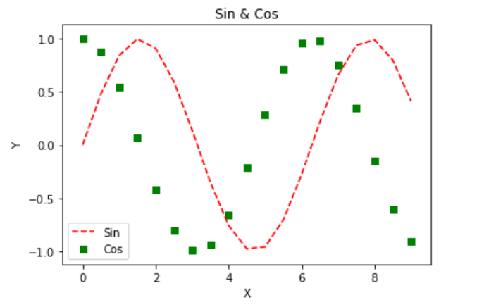
Plot
x=np.arange(0,3*np.pi,0.5)
y=np.sin(x)
z=np.cos(x)
plt.plot(x,y,'r--')
plt.scatter(x,z,c='g',marker=',')
plt.legend(('Sin','Cos'),loc='lower left')
plt.title('Sin & Cos')
plt.xlabel('X')
plt.ylabel('Y')
plt.show()
print: